This Project “RADAR RAINFALL MONITORING AND NOWCASTING SYSTEM FOR URBAN FLOOD MANAGEMENT IN SINGAPORE” is funded by PUB, Singapore. H2i (Hydroinformatics Institute) is going to hand over a peoduct including three X-band radars that cover Marina Catchment. The radar system consists of two essential parts, one is for rainfall observation, and the other is for nowcast. These two parts will be discussed in the following charpters.
The first question: How radar measures rainfall?
As we know, radar is capable of detecting the obstacle and bounce back the signal. With this analogy, rain drop above the ground will be detected by radar signals, and also drop size etc. Then the next thing left is to construct a relationship between radar reflectivity and rainfall rate, known as Z-R relashionshp, which will be covered in Z-R Relationship
Then we need to answer why radar?
Traditionally, we measure rainfall through some ground based devices, called gauge data. gauge data are usually considered as ground truth data. However, if the stakeholders need information like how is it possible to get inundated in city, or the government wants to alert citizens that there will be flooded, then gauge is of course not able to send off these signals. We need something more than ground! Here is why radar comes in to save lives!
Additionally, rain gauge data will not give you a full map of rain rate over a city, which means they are spatial constrained. But radar, on contrast, has a higher resolution over the domain and specialize at producing spatial rainfall rate.
After the mechanism explained, I would like to emphisize some limitations that radar would be confined or conditions where radar is not able to detect rainfall.
One severe problem for radar is that, its sight often get blocked by some skyscrapers especially in mega-cities.
Another problem is sometimes, radar imposes fake signals like clusters or non-precipitating dots.
In order to build a real-time radar monitoring system, more challenges is coming for the sake of computations. Appropriate algorithms should be selected for the tradeoff between accuracy and effort.
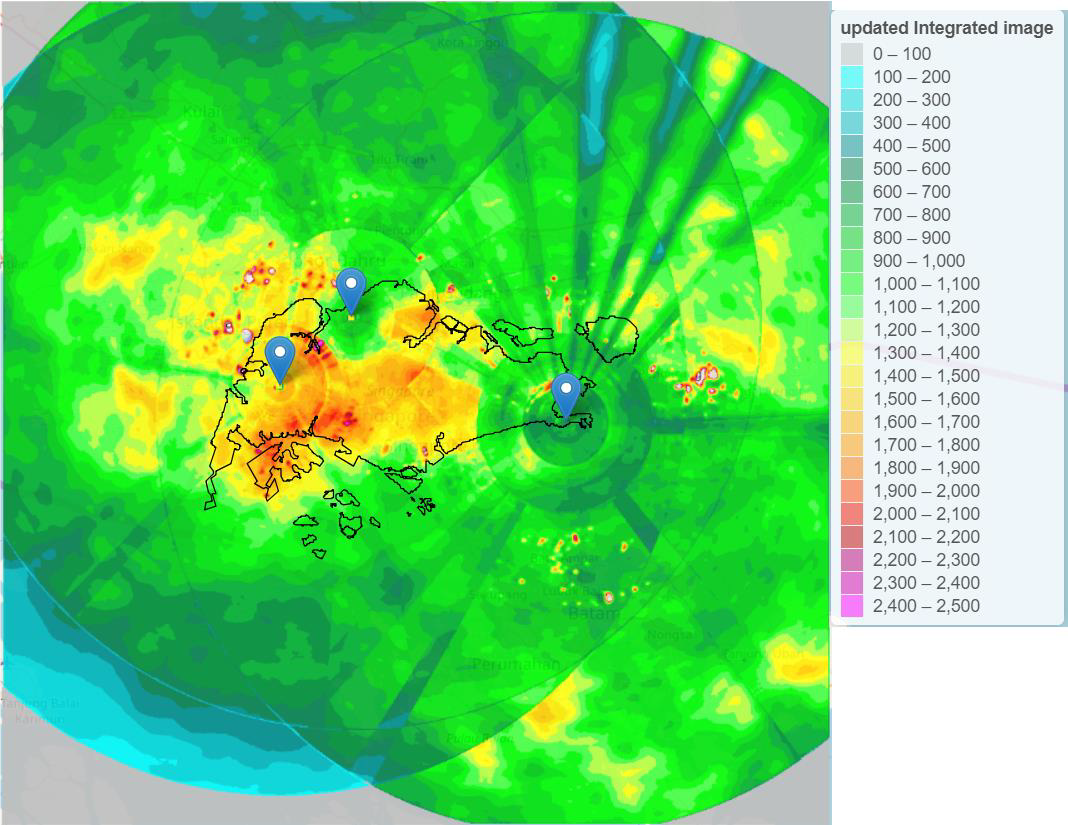
Three X-band radars are built in the western, eastern and norther part of Singapore, operating in observing rain and producing forecast every two minutes. Spatially, three radars will integrate together and produce a map with 100x100 meters resolution over 100kmx100km domain.
X-band radar contains around 9 layers of information, like rainfall, reflectivity, wind vector, etc. But in the first phase of this project, we only consider using reflectivity to calculate rainfall.
Z-R relationship directly maps reflectivity with rain rate. We construct this relationship based on emperial expression that has been provided with lots of practices.
\[Z=AR^b\]To calibrate this relationship, we selected several year-long events and calibrated the A, b parameter for each of three radar.
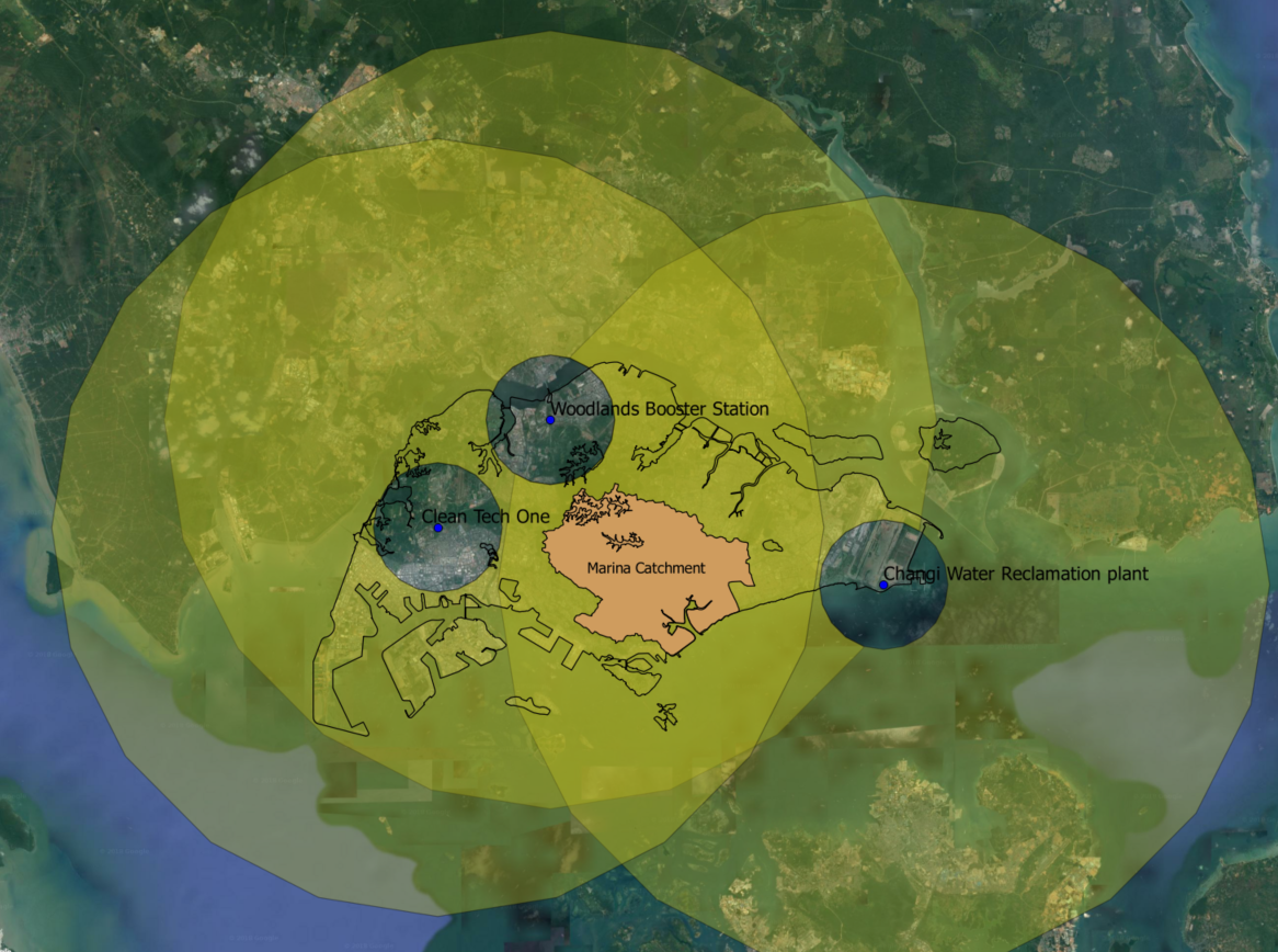
Three radars need to be integrated to produce only one spatially distributed rainfall map. Integration is based on maximizing the coverage of the radars. As described before, some radars fall into the poor sight, which means they are blocked by nearby buildings or telecommunications.
The figure above gives an illustrative example that one radar is blocked known as blind spots (radius)
To compensate for this, we analyzed the blind spots for each radar, and try to rely on each other to correct the blinds. Here we used weighted average value to determine which area is highly dependent on which radar.
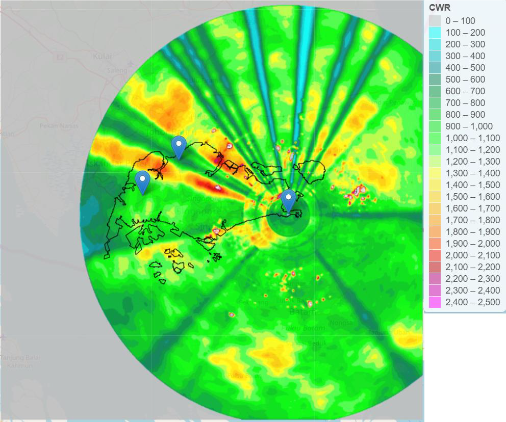
After this correction, the final map looks like this…
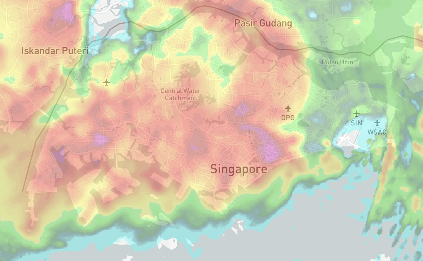
Radar nowcast plays an important role in releasing alert in the city if a potential flood is going to happen. The important signal for predicting rain over the large domain is relied on the movement of clouds.
With analogy to water quality model, the movement of clouds similarly will be decomposed as convection and diffusion.
Singapore, mostly suffers from convective storms, which simply conceptualize as decomposition of movement to velocity driven. Though this method is not accurate enough, it still supports us a big picture about where those rainy clouds to move.
The velocity for prediction is obtained by analyzing the movement of most clouds in the image domain. and then assume the persistence of Euler method, which freezes the last image (base image). After gaining information (velocity, moving direction), we forecast the cloud at next time step. With this method, we provide 45 minutes long-term forecasting in real-time(2 minutes latency).
Even though convective storm dominates over tropical regions like Singapore, the sophisticated atmosphiric model doesnot only account for 2-dimensional movement. As well, the growth and decay of the clouds should be taken into account. Since then, we propose a linear growth and decay model with following formula:
F_{T+i}^j=(C_i^1G_T^j+C_i^2R_T^j)/R_T^j
Memory integration comes into play because we observed the effect of previous velocity states. For instance, the continuity equation suggests that nothing will occur abruptly or dispear suddenly. This give us insights about using the combination of previous states of velocities to enhance our forecast model.
Obviously, there are bunch of ways to improve our existing radar performance. we will project to address these problems by alternating methods, even deep learning if possible.
In the future, we will be given more “reliable” data and not limited to ground proof gauge data. NEA will provide us another X-band radar data to better cross-validate data.
In such sense, to deal with multi-sourced data, it becomes obvious to utilize Kalman Filter for better data management.
Besides, we can also improve Z-R relationship with some machine learning techniques like Artificial Neural Network(ANN) or Random Forest (RF), but in my perspective, I prefer to use random forest because RF does not suffer from over-training, and should be enough to compensate all situations.
Meanwhile, if it is needed to clean radar raw data — reflectivity, we can train our data with autoencoder network before feeding into rainfall calculation. But I suspect that the training process and even evaluation will dramatically increase the calculation time. As for the real-time forecast, we may not be able to afford it.
Here is more appropriate to use deep learning model to forecast. It turns out some researches have been conducted in this topic. Mostly, LSTM (known as long short-term memory) fits into this topic, because it can recognize and memorize long sequence. Before actually implement this, I will post some repos on github to see the possibility.
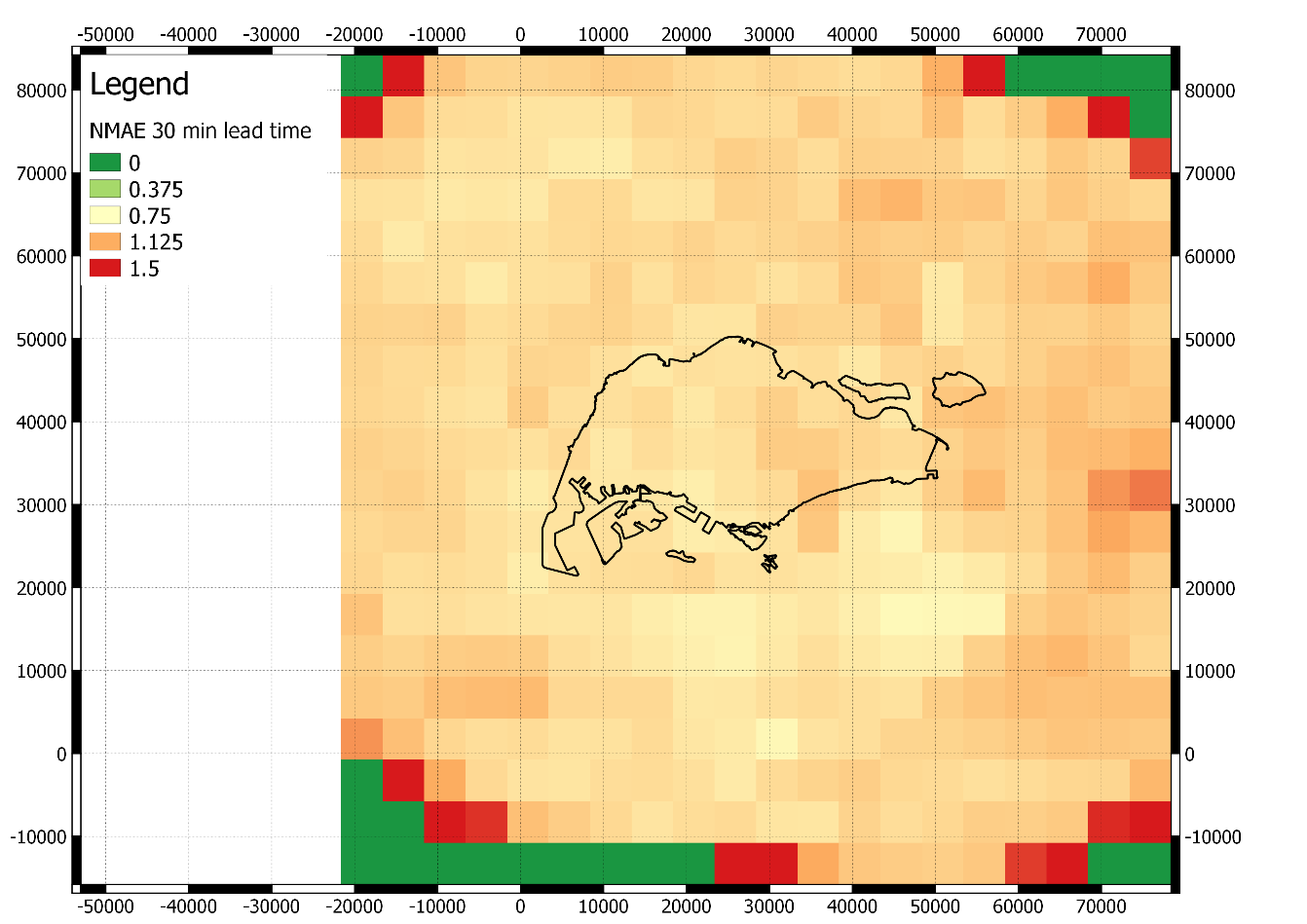
This chapter, I will introduce some statistical measurement used in this project, and also very wide-approached in the research. I will split this part into comparing with rain gauge which corresponds to point time series comparison and image comparison which is multi-dimensional statistics.
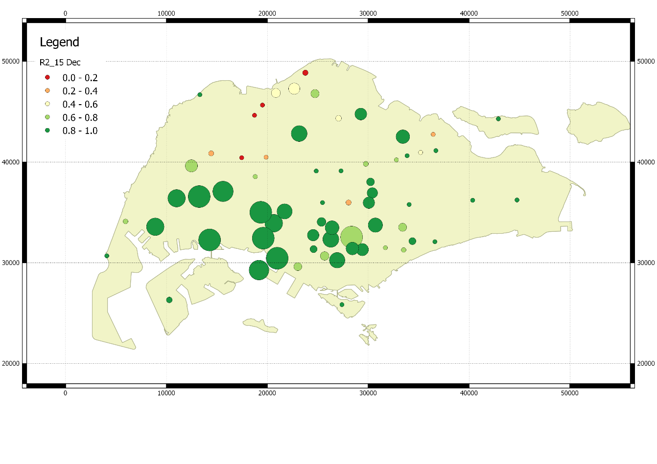
I believe everyone is familliar with this term RMSE. This should be introduced in high scholl when we measure how close two arrays are compared, like in calculating the variance.
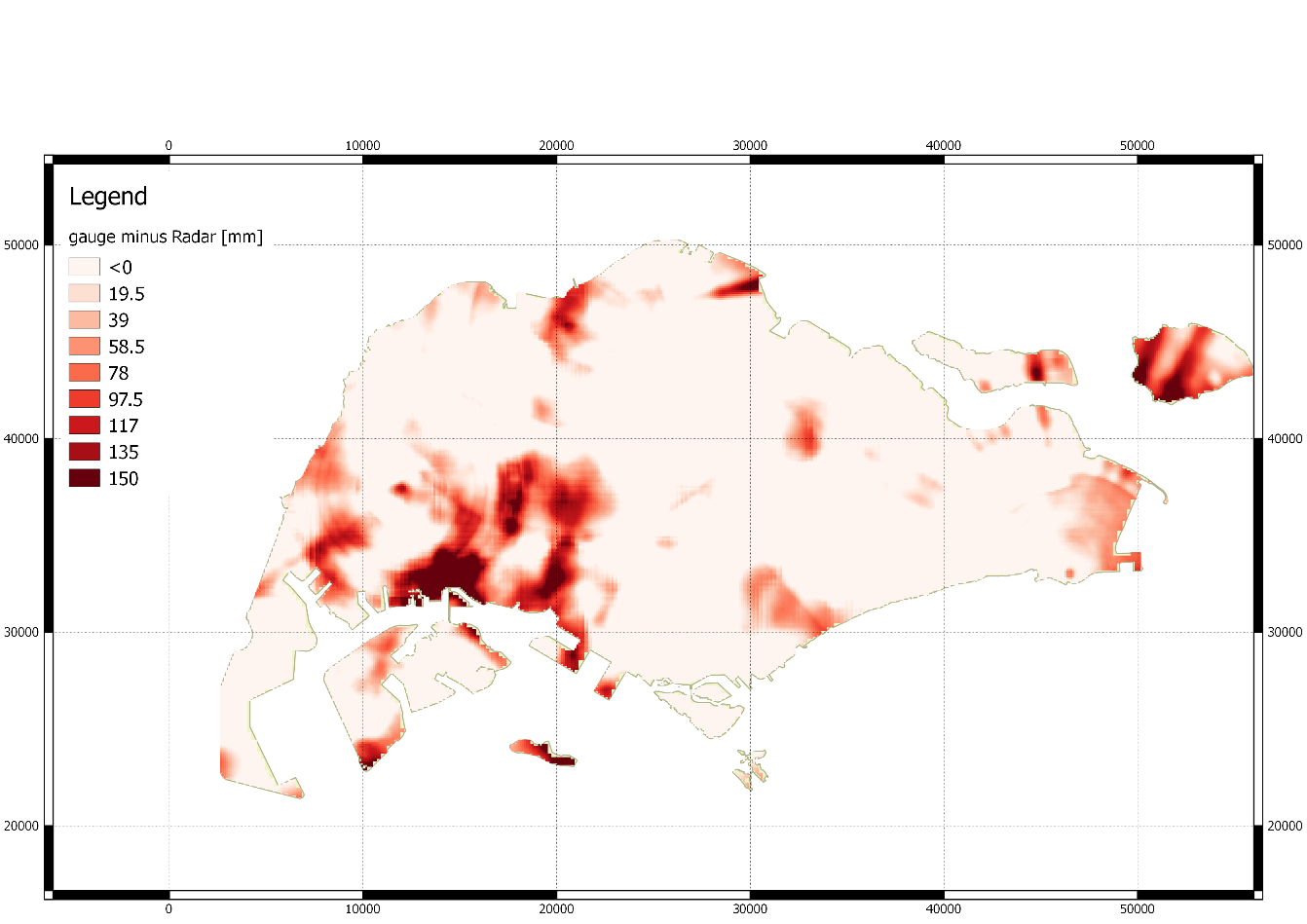
TVR is intuitively understandable. It compares the total rainfall observed by gauge and radar over a specific time duration (say an event). This statistic is useful when you want to emphisize whether radar is over-estimated or under-estimated. We mentioned that radar fails when it is blocked by high buildings, and typically in such regions, radar is underestimated comparing to gauge. Here we provide a good example showing the way to stress that radar is unreliable.
Again, this statistic is not complex. I will not explain it any further.
I want to make a point here that above statistics I mentioned have problem when accounting for different rainfall rate during event. For instance, one location falls more rainfall than other, would you expect this location has smaller error than other rain-free location?
Of course not, rain-free location has zero error but more rainfall brings with larger error. But the thing is, we donot care about rain-free areas, we only want to know how our rainfall measured by radar is close to gauge. Then we may need a trick — Normalized statistics.
Another technique here we discovered is that, these statistics are better during large events which means more rainfall, while worse during small rainfall. This will refer to the tipping bucket effect of gauge data. This graph to illustrate here is amazzzing…
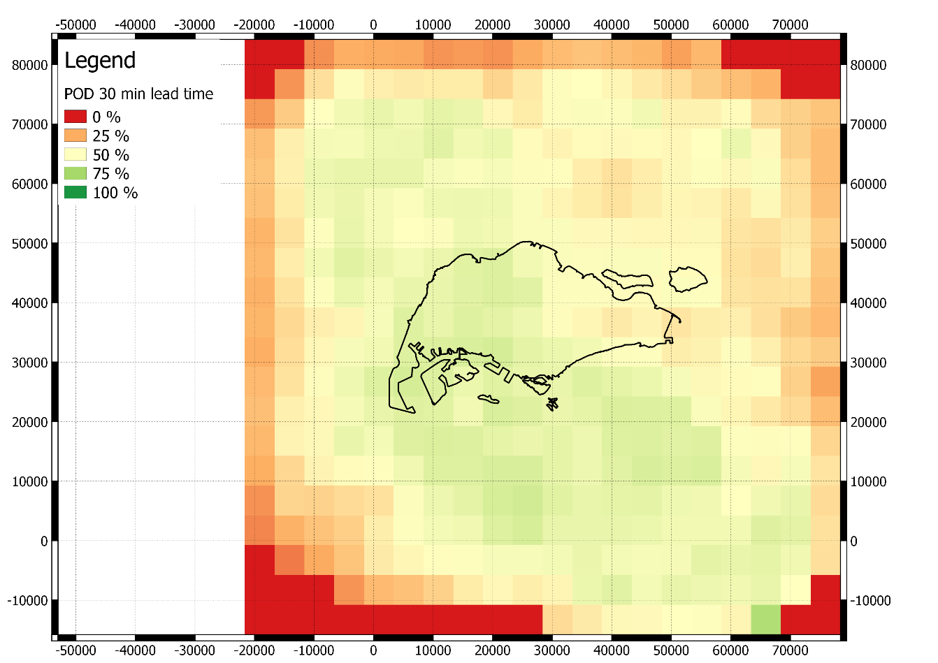
POD= \frac{a,a+b}
Where a is the number of grid cells where rain occurred and they were successful predicted as rain cells by the nowcasting model; and b is the number of grid cells where rain occurred but they were not predicted by the nowcasting model. What is marked as ‘rain’ and what as ‘no rain’ is determined using a particular threshold Z. The threshold is used because the measured radar data can have clutter and noise which can produce spurious values at low intensities. The threshold is set at Z = 0.5 mm/hr. This means that whenever rainfall is measured above this threshold it will be marked as an ‘rain’; otherwise as ‘no rain’.
| Measurement | Forecast rain | Forecast no-rain |
|---|---|---|
| Rain | a | b |
| no-rain | c | d |
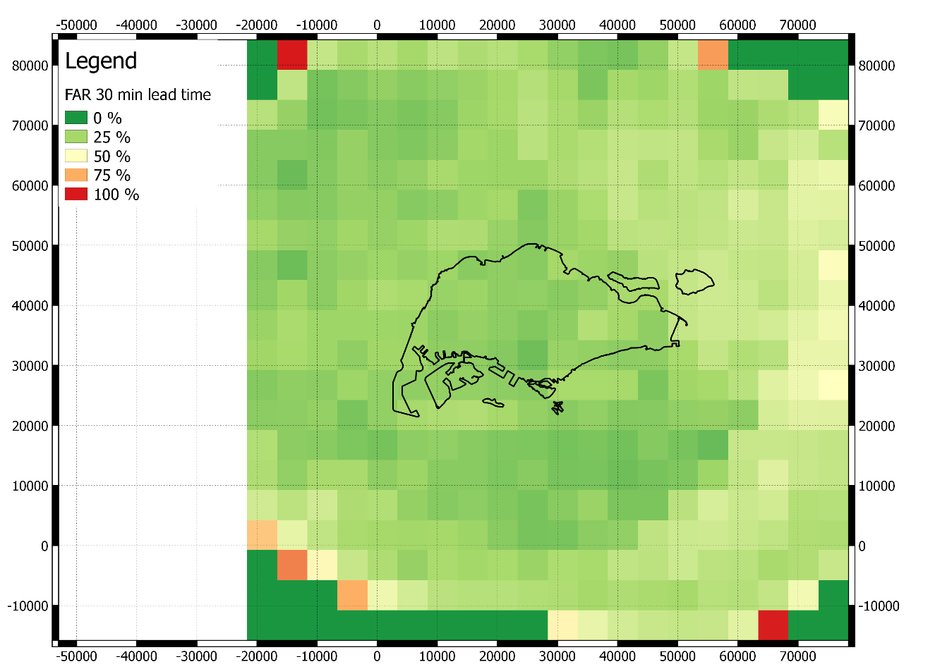
FAR= \frac{c,a+c}
where the a,c has the same meaning as before. This indicates the probability of producing false signal.
CSI=\frac{a, a+b+c}
where the a,b,c has the same meaning as before.